The concept of initial functor provides a categorical and operational semantics for equational reasoning with diagrams. So far, we have explored this thesis in the simplest possible setting, that of a bare category, or, in logical terms, of an equational theory with unary function symbols. This is rather restrictive. The standard setting for equational reasoning was historically the starting point of both categorical logic (Lawvere 1963) and e-graphs (Nelson 1980; Nelson and Oppen 1980): a category with finite products, viewed as an algebraic theory.
In this post, we extend the initial functor semantics from bare categories to categories with finite products. Surprisingly, this turns out to be, in a sense, trivial: the definition of initial functor need not be modified beyond asking that it preserve products. We can therefore jump straight into the rules of the formalism and an example calculation. Only in the final section, which is more technical, do we justify why the formalism need not be substantively changed from the unary setting.
1 Cartesian diagrams and term graphs
For our purposes, a category is cartesian if it has finite products, and a functor between cartesian categories is cartesian if it preserves finite products. A diagram D: \mathsf{J} \to \mathsf{C} in a cartesian category \mathsf{C} is cartesian if its shape \mathsf{J} is a cartesian category and the functor D is itself cartesian.
Cartesian categories and functors are familiar; cartesian diagrams less so, as limits or colimits are not usually indexed by categories assumed to have products. When taking limits in a cartesian category, there is no harm in taking the diagrams to be cartesian too, since a cone over a cartesian diagram is uniquely determined on its leg at a product of objects by its legs at each factor. This follows from the naturality of the cone with respect to product projections. Not only is there no harm in taking the diagram to be cartesian, it is important for us to do so since the diagram’s shape will encode systems of equations involving multiary operations.
The initial functor semantics has the virtue of being invariant: it does not depend on a particular way of presenting cartesian categories or cartesian diagrams. Even so, we often restrict to diagrams whose shapes are freely generated by a combinatorial structure. Such diagrams are syntactical in nature and resemble data structures used by computer scientists.
Recall that a free diagram is a diagram whose shape is a category freely generated by a graph. We say that a free cartesian diagram is a cartesian diagram whose shape is a cartesian category freely generated by a multigraph.1 There are several ways to explicitly describe the free cartesian category generated by a multigraph (see also Walters 1989), but we need not settle on one at this stage. The abstract characterization, given by the free-forgetful adjunction between cartesian categories and multigraphs, says that a free cartesian diagram D: F(M) \to \mathsf{C}, indexed by a multigraph M, is the same thing as a homomorphism2 M \to U(\mathsf{C}) from M into the underlying multigraph of \mathsf{C}. The latter is combinatorial data.
Under the logical perspective—that the objects and morphisms of a cartesian category \mathsf{C} are the types and operations of an algebraic theory—a free cartesian diagram in \mathsf{C} becomes a term graph over the algebraic theory. As formalized here,3 a term graph encodes terms as paths in a multigraph and, simultaneously, equations between terms by two or more multiedges incoming to a vertex. We illustrate this encoding through a toy example. Note that we draw term graphs differently than in the source material, in keeping with our different formalization of the concept.
Let \mathsf{C} be the signature with (i.e., the free cartesian category generated by) a type X and a binary operation {f: (X, X) \to X}. Then the terms f(a, b) and f(f(a, b), b) with free variables a: X and b: X, as well as the equation f(a, b) = a, can be encoded by the term graph (i.e., the free cartesian diagram) in \mathsf{C}:
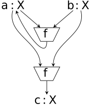
Due to the equation, the diagram includes redundant data. Later, we will see how to reduce it using congruence closure.
Note that, despite a superficial resemblance, cartesian diagrams are not string diagrams: they have no inputs or outputs, nor a preferred sense of direction.
In the operational semantics, morphisms between cartesian diagrams are more important than the diagrams themselves. Recall that a morphism of diagrams in a category \mathsf{C} is a functor between their shapes forming a commutative triangle over \mathsf{C}. In other words, the category of diagrams in \mathsf{C} is the slice \mathsf{Cat}/\mathsf{C}. A morphism of cartesian diagrams is a morphism of diagrams that is also cartesian as a functor; so, the category of cartesian diagrams in a cartesian category \mathsf{C} is the slice \mathsf{Cart}/\mathsf{C}.
2 Calculating with cartesian initial functors
We show how to derive equations using cartesian initial functors by first establishing the rules—themselves examples of cartesian initial functors—and then carrying out a small calculation. As hinted at the outset, a cartesian initial functor is nothing other than a functor that is both cartesian and initial.
2.1 Motifs among cartesian initial functors
We record a few important motifs, extending those in the first post to the cartesian setting. As in the second post, each motif is intended to be a rule of inference for diagrammatic reasoning.
Fix a cartesian category \mathsf{C}. To see that the functors below are initial, notice that pulling back along each one preserves limits; in fact, the limit of each diagram below is the product {X_1 \times \dots \times X_k} in \mathsf{C} (where k=4 in the final example).
Operation introduction: for any morphism f: (X_1, \dots, X_k) \to Y in \mathsf{C}, the map of cartesian diagrams
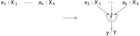
is initial.
Congruence reduction: for any morphism f: (X_1, \dots, X_k) \to Y in \mathsf{C}, the map of cartesian diagrams,
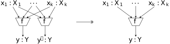
sending both y and y' on the left-hand side to y on the right-hand side, is initial.
Equation elimination: for any morphism f: (X_1, \dots, X_k) \to Y in \mathsf{C}, the map of cartesian diagrams
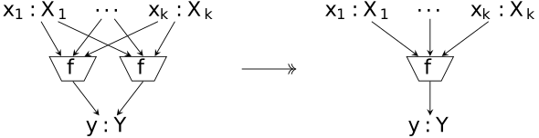
is initial.
Factorization: for any factorization of a morphism in \mathsf{C}, the map of cartesian diagrams from the diagram indexed by a single morphism to the diagram indexed by the shape of the factorization is initial. For example, given morphisms f: (X_1, X_2) \to Y_1,\quad g: (X_3, X_4) \to Y_2, \quad h: (Y_1, Y_2) \to Z in \mathsf{C}, the map of cartesian diagrams
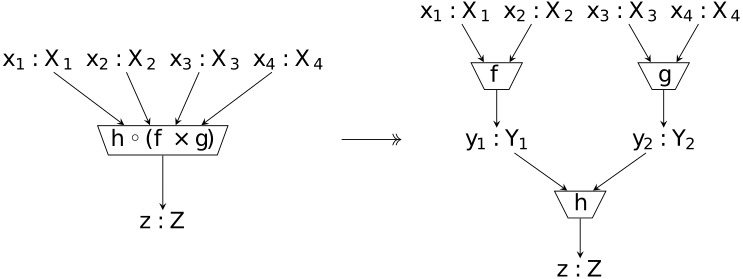
is initial.
Returning to the toy example, the morphism of cartesian diagrams,
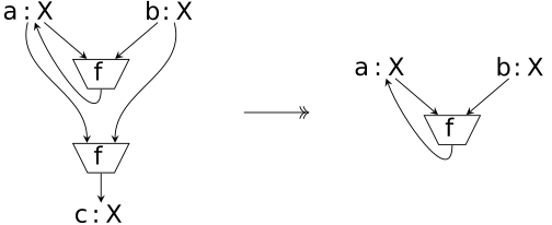
sending both a and c on the left-hand side to a on the right-hand side, is an initial functor. It is an application of congruence reduction. The diagram on the right cannot be reduced further.
Cyclic term graphs encode infinitely many terms in the same equivalence class. In this case, the terms f(a,b), f(f(a,b),b), f(f(f(a,b),b),b), \dots are all equivalent to a.
As before, we say that two cartesian diagrams D: \mathsf{J} \to \mathsf{C} and D': \mathsf{J}' \to \mathsf{C} are weakly equivalent, denoted D \sim D', if they can be connected by a zig-zag of morphisms, each of which is an initial functor. Weakly equivalent diagrams have the same limit, whenever the limit exists.
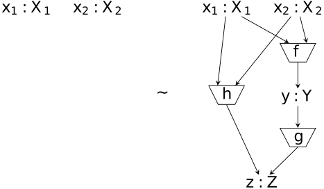
We can derive new rules—valid in the sense of preserving weak equivalence—by applying the motifs above in either direction. Particularly important is the equation introduction procedure for an equation between composite morphisms in the base category \mathsf{C}: starting with a discrete cartesian diagram, we apply operation introduction in the forward direction to the common composite; then equation elimination in the backward direction; and finally factorization twice in the forward direction, once for each side of the equation in \mathsf{C}. For example, suppose morphisms f: (X_1, X_2) \to Y, \quad g: Y \to Z, \quad h: (X_1, X_2) \to Z in \mathsf{C} satisfy h = g \circ f. Then there is a weak equivalence of cartesian diagrams:
2.2 A property of well-behaved lenses
Let \mathsf{C} be the algebraic theory of a well-behaved lens. Thus, \mathsf{C} is the algebraic theory with signature comprising
- basic types S (“source”) and V (“view”)
- operations \mathtt{get}: S \to V and \mathtt{put}: (S, V) \to S
and two axioms:
- PutGet: s: S,\, v: V \vdash \mathtt{get}(\mathtt{put}(s, v)) = v.
- GetPut: s: S \vdash \mathtt{put}(s, \mathtt{get}(s)) = s.
A very well-behaved or lawful lens satisfies the further property:
- PutPut: s: S,\, v,v': V \vdash \mathtt{put}(\mathtt{put}(s, v), v') = \mathtt{put}(s, v').
The PutPut law is independent of the other two. However, a special case of the PutPut equation, with v = v', is derivable from the first two laws:
- PutTwice: s: S,\, v: V \vdash \mathtt{put}(\mathtt{put}(s, v), v) = \mathtt{put}(s, v).
We are going to prove this by diagrammatic reasoning. In fact, the derivation is fairly trivial, but it is a known and noted fact in the lens literature (Fischer, Hu, and Pacheco 2015), and it illustrates the formalism.
Begin with the discrete cartesian diagram on S and V, representing the context s: S,\, v: V. Since the right-hand side of the target equation is \mathtt{put}(s, v), a natural first step is to introduce the \mathtt{put} operation:
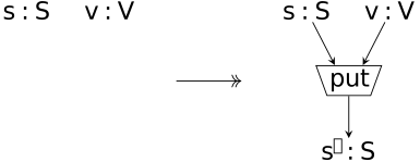
Recognizing a subterm of the PutGet law, introduce that equation at s and v too:
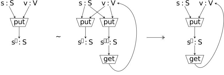
The morphism of diagrams on the right is a congruence reduction of \mathtt{put} at s and v. (We could have saved a few steps by immediately introducing the PutGet equation, but we wish to emphasize the mechanizability of such reasoning.) Next, we recognize a subterm of the GetPut law (replacing s with s'), so we introduce that equation at s':
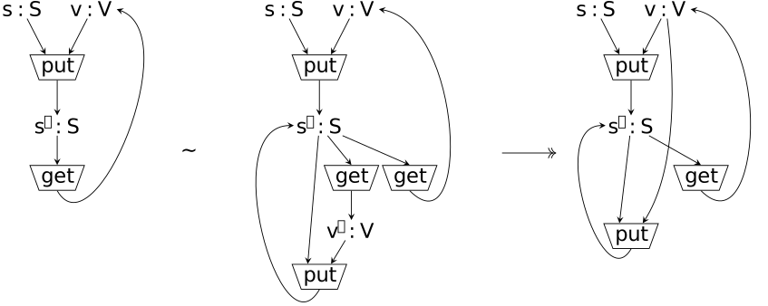
The final morphism of diagrams is again a congruence reduction, this time of \mathtt{get} at s'.
The resulting cartesian diagram contains the target equation, though it takes a moment to see that. Since the first and the last cartesian diagrams are weakly equivalent, and since the limit of the first diagram is the product {S \times V}, the limit of the last diagram is the same. Consequently, any two parallel paths in the last diagram starting at s and v compose to equal morphisms in \mathsf{C}. Taking the endpoint s' and following the cycle at s' (for fixed v) either zero times or once, we deduce the PutTwice law:
s: S,\, v: V \vdash \mathtt{put}(s, v) = \mathtt{put}(\mathtt{put}(s, v), v).
3 Comprehensive factorization for cartesian functors
As explained previously, the foundational theorem about initial functors is the existence of the comprehensive factorization system (Street and Walters 1973), an orthogonal factorization system on \mathsf{Cat} having initial functors and discrete opfibrations as its left and right classes. It turns out that the comprehensive factorization works just as well for cartesian functors as it does for arbitrary functors. This fact, possibly surprising, justifies our claim that the initial functor semantics carries over to the cartesian setting without modification. The precise statement is:
Theorem 1 (Comprehensive factorization on \mathsf{Cart}) The comprehensive factorization system on \mathsf{Cat} restricts to an orthogonal factorization system on \mathsf{Cart}, the category of small categories with finite products and finite-product-preserving functors.
We do not know a source for this theorem in the literature, though we presume it known since it follows straightforwardly from other, well-documented facts. In any case, the purpose of this section is to present a self-contained proof.
To prove the theorem, we show that the explicit construction of the comprehensive factorization, when applied to a cartesian functor, is a factorization in which the intermediate category and both functors are cartesian, without further assumptions. The analysis of the right class—discrete opfibrations—is simpler, so we start there.
3.1 Elements construction
Discrete opfibrations correspond to copresheaves via the elements construction. A simple result says that the elements construction preserves cartesianness.
Lemma 1 Let X: \mathsf{C} \to \mathsf{Set} be a cartesian set-valued functor on a cartesian category \mathsf{C}. Then its category of elements, \mathop{\mathsf{El}}(X), is cartesian, and its canonical projection, the discrete opfibration {\pi_X: \mathop{\mathsf{El}}(X) \to \mathsf{C}}, preserves and reflects finite products.
Proof. The product of objects (c_i, x_i)_{i \in I} in \mathop{\mathsf{El}}(X) is given, in its first component, by the product in \mathsf{C}, and, in its second component, by pairing:
\left( \prod_{i \in I} c_i,\ \langle x_i \rangle_{i \in I} \in \prod_{i \in I} X(c_i) \cong X\big({\textstyle\prod_{i \in I} c_i}\big) \right).
Product projections in \mathop{\mathsf{El}}(X) are simply the product projections in \mathsf{C}. The canonical projection \pi_X: {(c, x) \mapsto c},\, {f \mapsto f} clearly preserves finite products, and it also reflects them since a tuple is uniquely determined by its components.
3.2 Left Kan extension
Constructing the comprehensive factorization of a functor involves taking a left Kan extension, as we will review shortly. For now, the question is how left Kan extensions interact with finite products. The crucial concept in this analysis is siftedness—or rather its dual, cosiftedness. A textbook reference on sifted colimits is (Adámek, Rosický, and Vitale 2011, sec. I.2).
Definition 1 (Cosiftedness) A category \mathsf{J} is cosifted if any of the following equivalent conditions holds:
- in \mathsf{Set}, colimits of shape \mathsf{J}^\mathrm{op} commute with finite products;
- \mathsf{J} is nonempty and the diagonal \Delta_{\mathsf{J}}: \mathsf{J} \to \mathsf{J} \times \mathsf{J} is an initial functor;
- \mathsf{J} is nonempty and for any objects j_1, j_2 \in \mathsf{J}, the category \mathsf{Span}_{\mathsf{J}}(j_1, j_2) of spans in \mathsf{J} with feet j_1 and j_2 is nonempty and connected.
A cosifted colimit is a colimit whose shape is a cosifted category.
Lemma 2 A category with finite products is cosifted.
Proof. Suppose \mathsf{J} has finite products. Then \mathsf{J} is nonempty, having a terminal object, and for any objects j_1, j_2 \in \mathsf{J}, the category \mathsf{Span}_{\mathsf{J}}(j_1, j_2) has a terminal object—the product cone {j_1 \leftarrow j_1 \times j_2 \to j_2}, by the universal property of the product—so is in particular nonempty and connected.
The surprising fact is that the left Kan extension of a cartesian set-valued functor along any functor (not necessarily cartesian) is again cartesian. This result first appears in the literature as (Borceux and Day 1977, Theorem 1.5 and Example 3.1), in the more general setting of enriched categories. We give a direct and elementary proof.
Theorem 2 (Product-preserving Kan extensions) Let \mathsf{C} and \mathsf{D} be cartesian categories, and let X: \mathsf{C} \to \mathsf{Set} be a cartesian set-valued functor. For any functor F: \mathsf{C} \to \mathsf{D}, the left Kan extension \operatorname{Lan}_F X: \mathsf{D} \to \mathsf{Set} is cartesian.
Proof. Decomposing X as a canonical colimit of representables, the left Kan extension of X has the formula:
\operatorname{Lan}_F X \cong \mathop{\mathrm{colim}}_{(c,x) \in {\mathop{\mathsf{El}}(X)}^\mathrm{op}} \mathsf{D}(F(c), -).
Because the representables \mathsf{D}(F(c), -): \mathsf{D} \to \mathsf{Set} preserve finite products, \operatorname{Lan}_F X will preserve finite products when \mathop{\mathsf{El}}(X) is cosifted. But that is the case by Lemma 1 and Lemma 2.
3.3 Proof of the theorem
We now have all the ingredients we need to prove Theorem 1, that the comprehensive factorization on \mathsf{Cat} restricts to \mathsf{Cart}, the category of cartesian categories and cartesian functors.
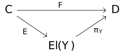
To do this, we look inside the proof of (Street and Walters 1973, Theorem 3) at how the comprehensive factorization of a functor F: \mathsf{C} \to \mathsf{D} is constructed. Let X: \mathsf{C} \to \mathsf{Set},\, c \mapsto 1 be the terminal copresheaf, and take its left Kan extension along F, yielding a copresheaf {Y \mathrel{\vcenter{:}}=\operatorname{Lan}_F X}. By the universal property of the category of elements as a comma category, {\mathop{\mathsf{El}}(Y) = 1/Y}, there exists a unique functor {E: \mathsf{C} \to \mathop{\mathsf{El}}(Y)} factorizing F as
and equating the 2-cells:
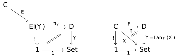
In this factorization, \pi_Y is a discrete opfibration, and Street and Walters (1973) show that E is initial. So {F = \pi_Y \circ E} is the comprehensive factorization of F.
Now, if \mathsf{C} and \mathsf{D} are cartesian, then so is X, since 1 \times 1 \cong 1; hence, so is Y = \operatorname{Lan}_F X, by Theorem 2 on product-preserving Kan extensions; hence, so are \mathop{\mathsf{El}}(Y) and \pi_Y by Lemma 1. Moreover, if F is also cartesian, then so is E, since the composite {\pi_Y \circ E = F} preserves finite products and, by Lemma 1, \pi_Y reflects them. Thus, the factorization {F = \pi_Y \circ E} in \mathsf{Cat} restricts to \mathsf{Cart}. This completes the proof, using the characterization of a factorization system in terms of unique factorization up to unique isomorphism.
4 Outlook
We’ve seen how the initial functor semantics extends from bare categories to categories with finite products, the classical setting for both categorical logic and e-graphs. The generalization is illustrated by example calculations and justified by the theoretical result that the comprehensive factorization works just as well for product-preserving functors.
A potential benefit of a categorical semantics is suggesting further generalizations of e-graph-style reasoning to new or nonstandard settings. The theoretical analysis here suggests both opportunities and challenges in this regard. On one hand, it seems likely that the cartesian version of the comprehensive factorization will generalize to cartesian equipments or, what are closely related, fibrations of cartesian categories. These categorical structures correspond to an enhanced kind of algebraic theory having first-class functions and relations, as found in the recent system egglog. On the other hand, the comprehensive factorization system will not directly extend from categories with finite products to categories with all finite limits, corresponding to essentially algebraic or generalized algebraic theories (GATs). To make this work, the concept of a flat functor might need to enter the picture. We will consider such extensions in the future.
5 References
Footnotes
Be warned that we use the category theorist’s terminology, not the graph theorist’s. So a graph is what a graph theorist might call a “directed multigraph (with self-loops).” Meanwhile, a multigraph is a combinatorial structure consisting of a set of vertices and a set of multiedges, where each multiedge is assigned a source, a list of vertices, as well as a target, a single vertex. The arity of a multiedge is the length of the list that is its source. With this terminology, graphs are to categories as multigraphs are to multicategories.↩︎
A morphism of multigraphs consists of a pair of functions between the vertex and multiedge sets, preserving the source and target assignments. In particular, preserving sources includes the requirement that arities are preserved.↩︎
Though long used in computer science, term graphs have often been formalized with less than perfect clarity. Nelson (1980, sec. 6) defines an equality graph or e-graph, a kind of term graph, to be a graph whose vertices are labeled by variables or function symbols and whose edges are a (totally?) ordered set. This global ordering induces a local ordering of the edges incoming to each vertex. A term graph is better defined as a labeled multigraph, i.e., as a multigraph homomorphism into a fixed multigraph.↩︎